Load the R package we will use.

library(tidyverse)
library(infer)
library(skimr)

Make sure you have installed and loaded the tidyverse, infer, and skimr packages
Fill in the blanks
Put the command you use in the Rchunks in your Rmd file for this quiz.

T-Test

The data this quiz is a subset of HR
- Look at the variable definitions
- Note that the variables evaluation and salary have been recoded to be represented as words instead of numbers
Set random seed generator to 123

set.seed(123)

hr_1_tidy.csv is the name of your data subset
Read it into and assign to hr
- Note: col_types = “fddfff” defines the column types factor-double-double-factor-factor-factor

hr  <- read_csv("https://estanny.com/static/week13/data/hr_1_tidy.csv", 
                col_types = "fddfff")

Use skim to summarize the data in hr

skim(hr)

Table 1: Data summary
Name	hr
Number of rows	500
Number of columns	6
_______________________
Column type frequency:
factor	4
numeric	2
________________________
Group variables	None

Variable type: factor

skim_variable	complete_rate	ordered	n_unique	top_counts
gender	1	FALSE	2	fem: 260, mal: 240
evaluation	1	FALSE	4	bad: 153, fai: 142, goo: 106, ver: 99
salary	1	FALSE	6	lev: 93, lev: 92, lev: 91, lev: 84
status	1	FALSE	3	fir: 185, pro: 162, ok: 153

Variable type: numeric

skim_variable	n_missing	complete_rate	mean	sd	p0	p25	p50	p75	p100	hist
age	0	1	40.60	11.58	20.2	30.37	41.00	50.82	59.9	▇▇▇▇▇
hours	0	1	49.32	13.13	35.0	37.55	45.25	58.45	79.7	▇▂▃▂▂

specify that hours is the variable of interest

hr  %>% 
  specify(response = hours)

Response: hours (numeric)
# A tibble: 500 × 1
   hours
   <dbl>
 1  36.5
 2  55.8
 3  35  
 4  52  
 5  35.1
 6  36.3
 7  40.1
 8  42.7
 9  66.6
10  35.5
# … with 490 more rows

hypothesize that the average hours worked is 48

hr  %>% 
  specify(response = hours)  %>% 
  hypothesize(null = "point", mu = 48)

Response: hours (numeric)
Null Hypothesis: point
# A tibble: 500 × 1
   hours
   <dbl>
 1  36.5
 2  55.8
 3  35  
 4  52  
 5  35.1
 6  36.3
 7  40.1
 8  42.7
 9  66.6
10  35.5
# … with 490 more rows

generate 1000 replicates representing the null hypothesis

hr %>% 
  specify(response = hours)  %>% 
  hypothesize(null = "point", mu = 48)  %>% 
  generate(reps = 1000, type = "bootstrap")

Response: hours (numeric)
Null Hypothesis: point
# A tibble: 500,000 × 2
# Groups:   replicate [1,000]
   replicate hours
       <int> <dbl>
 1         1  33.7
 2         1  34.9
 3         1  46.6
 4         1  33.8
 5         1  61.2
 6         1  34.7
 7         1  37.9
 8         1  39.0
 9         1  62.8
10         1  50.9
# … with 499,990 more rows

calculate the distribution of statistics from the generated data

Assign the output null_t_distribution
Display null_t_distribution

null_t_distribution  <- hr  %>% 
  specify(response = age)  %>% 
  hypothesize(null = "point", mu = 48)  %>% 
  generate(reps = 1000, type = "bootstrap")  %>% 
  calculate(stat = "t")

null_t_distribution

Response: age (numeric)
Null Hypothesis: point
# A tibble: 1,000 × 2
   replicate   stat
       <int>  <dbl>
 1         1  0.802
 2         2 -0.706
 3         3  1.33 
 4         4 -0.245
 5         5 -1.11 
 6         6  0.382
 7         7 -0.904
 8         8  0.816
 9         9  0.968
10        10  0.979
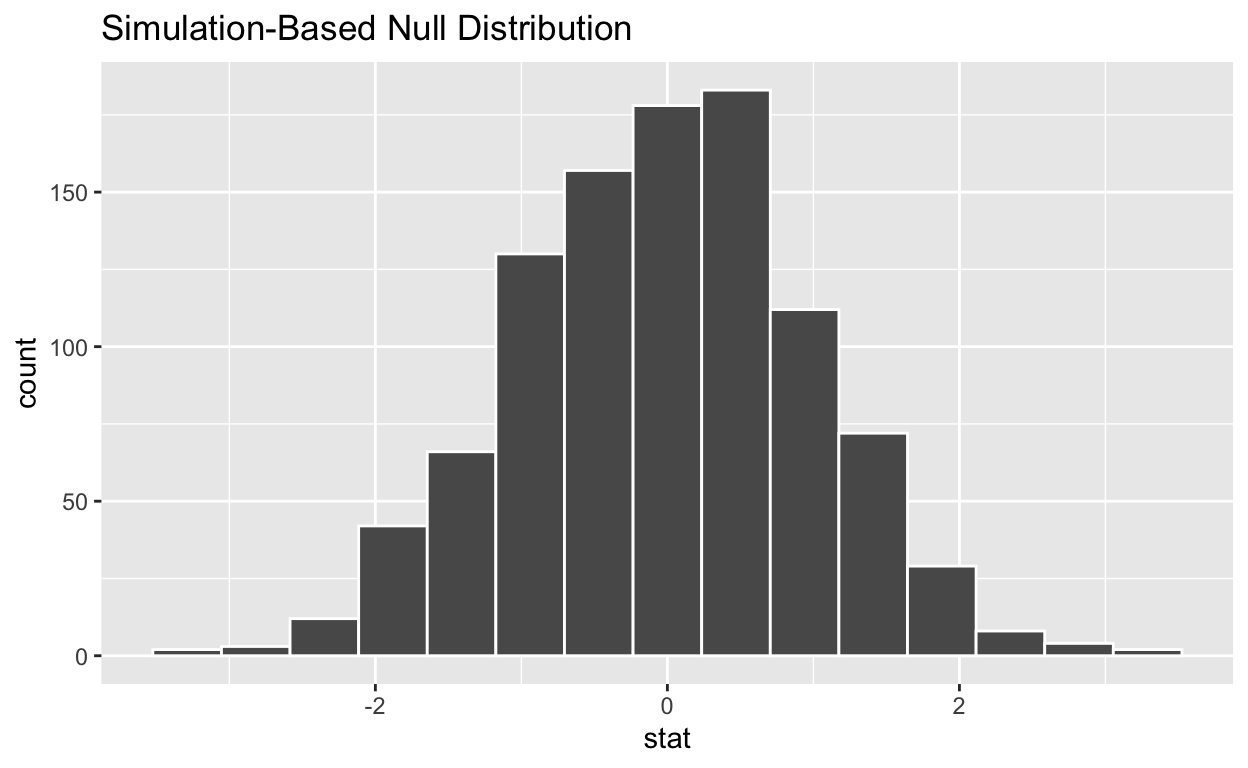
# … with 990 more rows

visualize the simulated null distribution

visualize(null_t_distribution)

calculate the statistic from your observed data

Assign the output observed_t_statistic
Display observed_t_statistic

observed_t_statistic  <- hr  %>%
  specify(response = hours)  %>% 
  hypothesize(null = "point", mu = 48)  %>%
  calculate(stat = "t")

observed_t_statistic

Response: hours (numeric)
Null Hypothesis: point
# A tibble: 1 × 1
   stat
  <dbl>
1  2.25

get_p_value from the simulated null distribution and the observed statistic

null_t_distribution  %>% 
  get_p_value(obs_stat = observed_t_statistic, direction = "two-sided")

# A tibble: 1 × 1
  p_value
    <dbl>
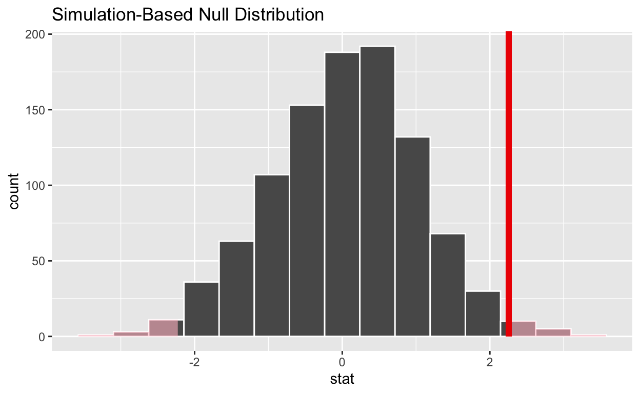
1   0.022

shade_p_value on the simulated null distribution

null_t_distribution  %>% 
  visualize() +
  shade_p_value(obs_stat = observed_t_statistic, direction = "two-sided")

Make sure you have installed and loaded the tidyverse, infer, and skimr packages
Fill in the blanks
Put the command you use in the Rchunks in your Rmd file for this quiz.
The data this quiz is a subset of HR
- Look at the variable definitions
- Note that the variables evaluation and salary have been recoded to be represented as words instead of numbers

hr_1_tidy.csv is the name of your data subset

Read it into and assign to hr_2
- Note: col_types = “fddfff” defines the column types factor-double-double-factor-factor-factor

hr_2 <- read_csv("https://estanny.com/static/week13/data/hr_2_tidy.csv", 
                col_types = "fddfff")

Is the average number of hours worked the same for both genders in hr_2

use skim to summarize the data in hr_2 by gender

hr_2 %>% 
  group_by(gender)  %>% 
  skim()

Table 2: Data summary
Name	Piped data
Number of rows	500
Number of columns	6
_______________________
Column type frequency:
factor	3
numeric	2
________________________
Group variables	gender

Variable type: factor

skim_variable	gender	complete_rate	ordered	n_unique	top_counts
evaluation	male	1	FALSE	4	bad: 79, fai: 68, goo: 61, ver: 48
evaluation	female	1	FALSE	4	bad: 75, fai: 74, ver: 48, goo: 47
salary	male	1	FALSE	6	lev: 49, lev: 48, lev: 48, lev: 44
salary	female	1	FALSE	6	lev: 47, lev: 46, lev: 41, lev: 39
status	male	1	FALSE	3	fir: 93, pro: 90, ok: 73
status	female	1	FALSE	3	fir: 101, pro: 89, ok: 54

Variable type: numeric

skim_variable	gender	complete_rate	mean	sd	p0	p25	p50	p75	p100	hist
age	male	1	38.63	11.57	20.3	28.50	37.85	49.52	59.6	▇▇▆▆▆
age	female	1	41.14	11.43	20.3	31.30	41.60	50.90	59.9	▆▅▇▇▇
hours	male	1	49.30	13.24	35.0	37.35	46.00	59.23	79.9	▇▃▂▂▂
hours	female	1	49.49	13.08	35.0	37.68	45.05	58.73	78.4	▇▃▃▂▂

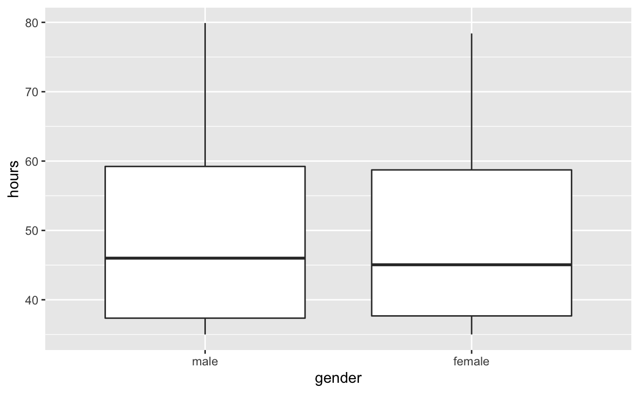
Use geom_boxplot to plot distributions of hours worked by gender

hr_2 %>% 
  ggplot(aes(x = gender, y = hours)) + 
  geom_boxplot()

specify the variables of interest are hours and gender

hr_2 %>% 
  specify(response = hours, explanatory = gender)

Response: hours (numeric)
Explanatory: gender (factor)
# A tibble: 500 × 2
   hours gender
   <dbl> <fct> 
 1  78.1 male  
 2  35.1 female
 3  36.9 female
 4  38.5 male  
 5  36.1 male  
 6  78.1 female
 7  76   female
 8  35.6 female
 9  35.6 male  
10  56.8 male  
# … with 490 more rows

hypothesize that the number of hours worked and gender are independent

hr_2  %>% 
  specify(response = hours, explanatory = gender)  %>% 
  hypothesize(null = "independence")

Response: hours (numeric)
Explanatory: gender (factor)
Null Hypothesis: independence
# A tibble: 500 × 2
   hours gender
   <dbl> <fct> 
 1  78.1 male  
 2  35.1 female
 3  36.9 female
 4  38.5 male  
 5  36.1 male  
 6  78.1 female
 7  76   female
 8  35.6 female
 9  35.6 male  
10  56.8 male  
# … with 490 more rows

generate 1000 replicates representing the null hypothesis

hr_2 %>% 
  specify(response = hours, explanatory = gender)  %>% 
  hypothesize(null = "independence")  %>% 
  generate(reps = 1000, type = "permute")

Response: hours (numeric)
Explanatory: gender (factor)
Null Hypothesis: independence
# A tibble: 500,000 × 3
# Groups:   replicate [1,000]
   hours gender replicate
   <dbl> <fct>      <int>
 1  47.8 male           1
 2  60.3 female         1
 3  46.5 female         1
 4  37.2 male           1
 5  74.1 male           1
 6  35.9 female         1
 7  35.6 female         1
 8  54.5 female         1
 9  55.6 male           1
10  44.1 male           1
# … with 499,990 more rows

calculate the distribution of statistics from the generated data

- Assign the output null_distribution_2_sample_permute

- Display         null_distribution_2_sample_permute

null_distribution_2_sample_permute  <- hr_2 %>% 
  specify(response = hours, explanatory = gender)  %>% 
  hypothesize(null = "independence")  %>% 
  generate(reps = 1000, type = "permute")  %>% 
  calculate(stat = "t", order = c("female", "male"))

null_distribution_2_sample_permute

Response: hours (numeric)
Explanatory: gender (factor)
Null Hypothesis: independence
# A tibble: 1,000 × 2
   replicate   stat
       <int>  <dbl>
 1         1  0.505
 2         2 -0.650
 3         3  0.279
 4         4  0.435
 5         5  1.73 
 6         6 -0.139
 7         7 -2.14 
 8         8  0.274
 9         9  0.766
10        10  1.52 
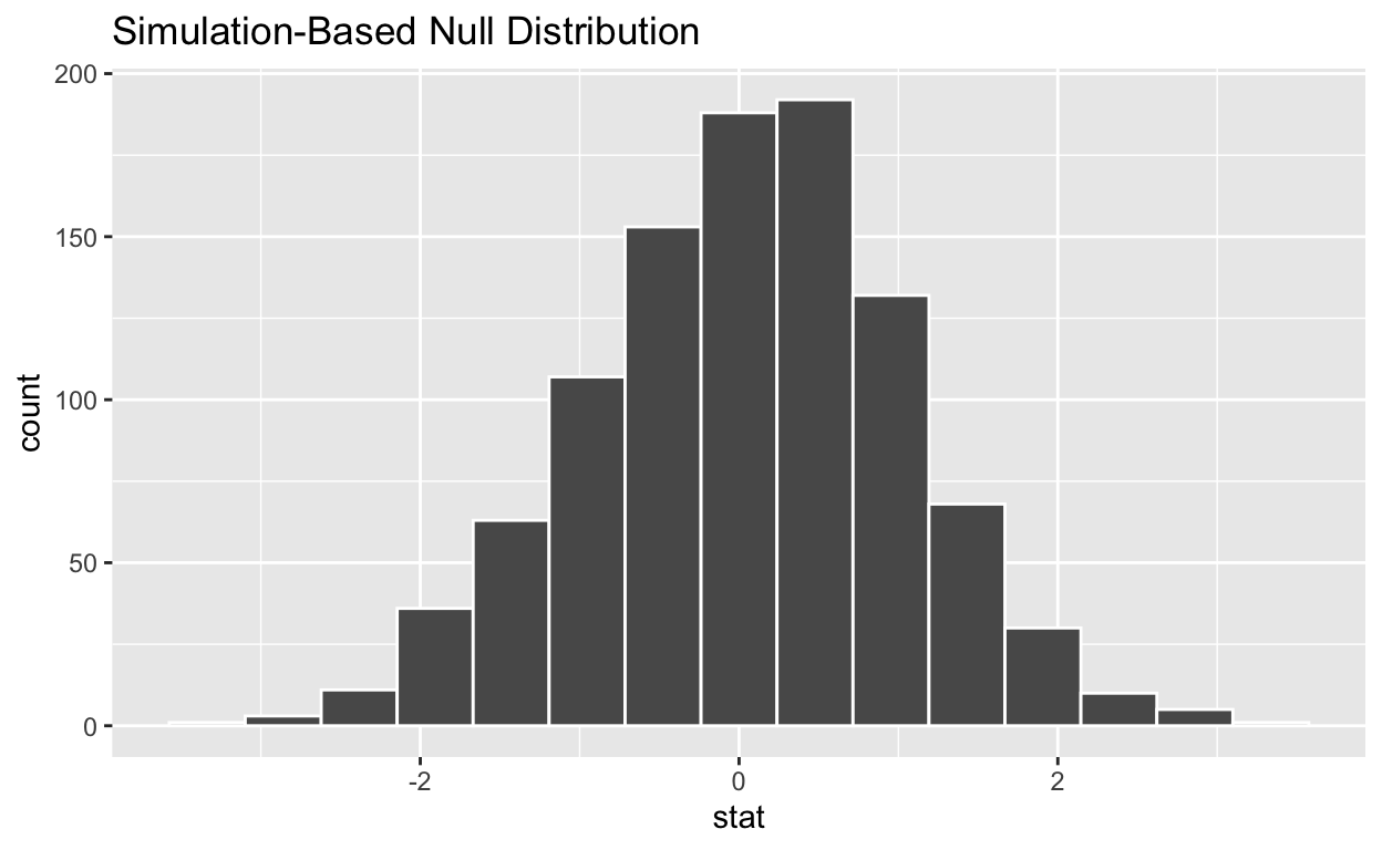
# … with 990 more rows

visualize the simulated null distribution

visualize(null_distribution_2_sample_permute)

calculate the statistic from your observed data
Assign the output observed_t_2_sample_stat
Display observed_t_2_sample_stat

observed_t_2_sample_stat  <- hr_2 %>%
  specify(response = hours, explanatory = gender)  %>% 
  calculate(stat = "t", order = c("female", "male"))

observed_t_2_sample_stat

Response: hours (numeric)
Explanatory: gender (factor)
# A tibble: 1 × 1
   stat
  <dbl>
1 0.160

get_p_value from the simulated null distribution and the observed statistic

null_t_distribution  %>% 
  get_p_value(obs_stat = observed_t_2_sample_stat, direction = "two-sided")

# A tibble: 1 × 1
  p_value
    <dbl>
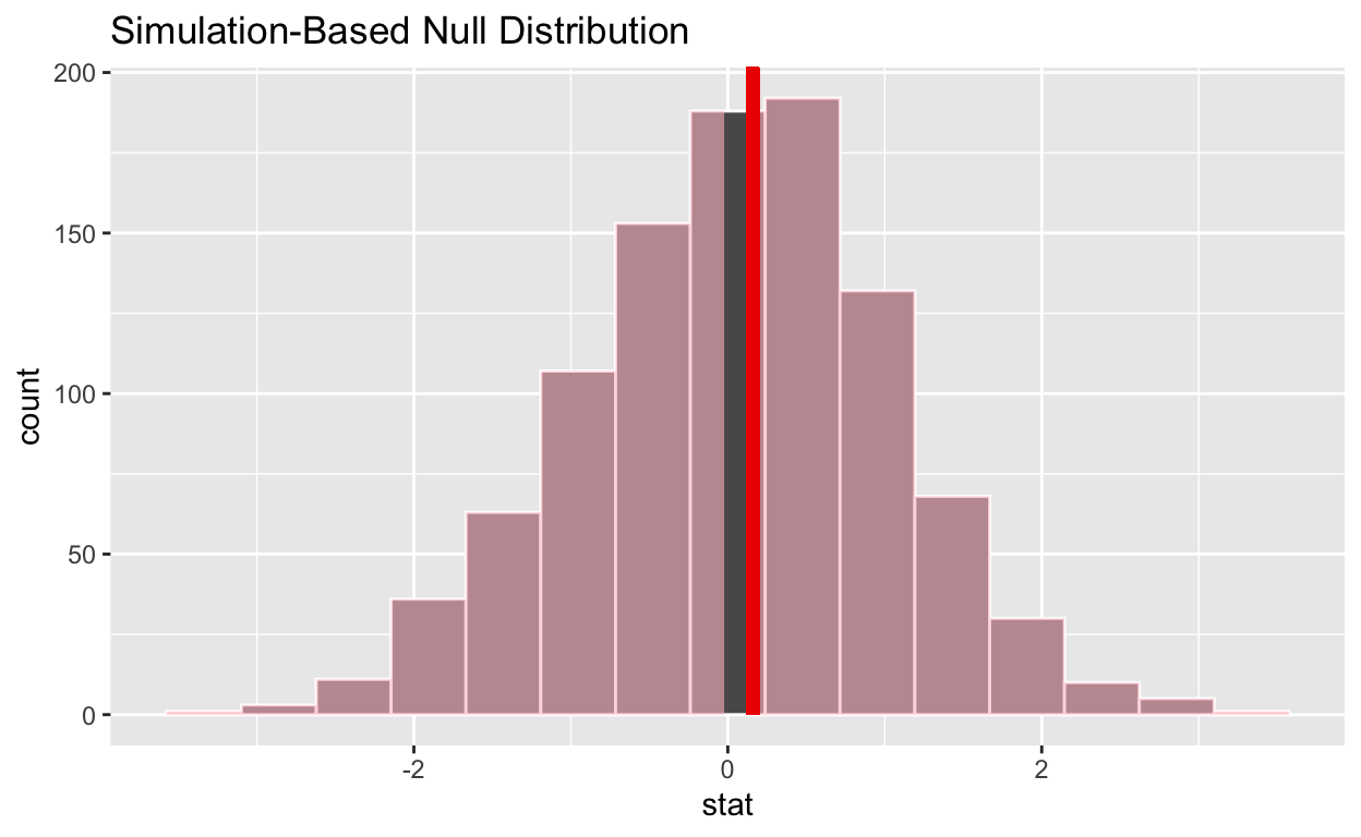
1   0.918

shade_p_value on the simulated null distribution

null_t_distribution  %>% 
  visualize() +
  shade_p_value(obs_stat = observed_t_2_sample_stat, direction = "two-sided")

Make sure you have installed and loaded the tidyverse, infer, and skimr packages
Fill in the blanks
Put the command you use in the Rchunks in your Rmd file for this quiz.
The data this quiz is a subset of HR
- Look at the variable definitions
- Note that the variables evaluation and salary have been recoded to be represented as words instead of numbers
hr_2_tidy.csv is the name of your data subset
Read it into and assign to hr_anova
- Note: col_types = “fddfff” defines the column types factor-double-double-factor-factor-factor

hr_anova <- read_csv("https://estanny.com/static/week13/data/hr_2_tidy.csv", 
                col_types = "fddfff")

Q: Is the average number of hours worked the same for all three status (fired, ok and promoted) ?

use skim to summarize the data in hr_anova by status

hr_anova %>% 
  group_by(status)  %>% 
  skim()

Table 3: Data summary
Name	Piped data
Number of rows	500
Number of columns	6
_______________________
Column type frequency:
factor	3
numeric	2
________________________
Group variables	status

Variable type: factor

skim_variable	status	complete_rate	ordered	n_unique	top_counts
gender	promoted	1	FALSE	2	mal: 90, fem: 89
gender	fired	1	FALSE	2	fem: 101, mal: 93
gender	ok	1	FALSE	2	mal: 73, fem: 54
evaluation	promoted	1	FALSE	4	goo: 70, ver: 62, fai: 24, bad: 23
evaluation	fired	1	FALSE	4	bad: 78, fai: 72, goo: 25, ver: 19
evaluation	ok	1	FALSE	4	bad: 53, fai: 46, ver: 15, goo: 13
salary	promoted	1	FALSE	6	lev: 42, lev: 42, lev: 39, lev: 34
salary	fired	1	FALSE	6	lev: 54, lev: 44, lev: 34, lev: 24
salary	ok	1	FALSE	6	lev: 32, lev: 31, lev: 26, lev: 19

Variable type: numeric

skim_variable	status	complete_rate	mean	sd	p0	p25	p50	p75	p100	hist
age	promoted	1	40.63	11.25	20.4	30.75	41.10	50.25	59.9	▆▇▇▇▇
age	fired	1	40.03	11.53	20.3	29.45	40.40	50.08	59.9	▇▅▇▆▆
age	ok	1	38.50	11.98	20.3	28.15	38.70	49.45	59.9	▇▆▅▅▆
hours	promoted	1	59.21	12.66	35.0	49.75	58.90	70.65	79.9	▅▆▇▇▇
hours	fired	1	41.67	8.37	35.0	36.10	38.45	43.40	77.7	▇▂▁▁▁
hours	ok	1	47.35	10.86	35.0	37.10	45.70	54.50	78.9	▇▅▃▂▁

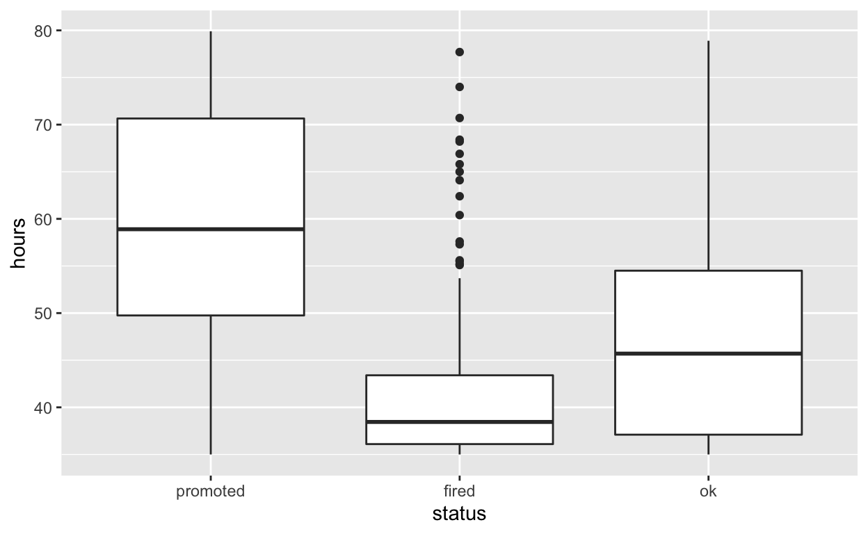
Use geom_boxplot to plot distributions of hours worked by status

hr_anova %>% 
  ggplot(aes(x = status, y = hours)) + 
  geom_boxplot()

specify the variables of interest are hours and status

hr_anova %>% 
  specify(response = hours, explanatory = status)

Response: hours (numeric)
Explanatory: status (factor)
# A tibble: 500 × 2
   hours status  
   <dbl> <fct>   
 1  78.1 promoted
 2  35.1 fired   
 3  36.9 fired   
 4  38.5 fired   
 5  36.1 fired   
 6  78.1 promoted
 7  76   promoted
 8  35.6 fired   
 9  35.6 ok      
10  56.8 promoted
# … with 490 more rows

hypothesize that the number of hours worked and status are independent

hr_anova  %>% 
  specify(response = hours, explanatory = status)  %>% 
  hypothesize(null = "independence")

Response: hours (numeric)
Explanatory: status (factor)
Null Hypothesis: independence
# A tibble: 500 × 2
   hours status  
   <dbl> <fct>   
 1  78.1 promoted
 2  35.1 fired   
 3  36.9 fired   
 4  38.5 fired   
 5  36.1 fired   
 6  78.1 promoted
 7  76   promoted
 8  35.6 fired   
 9  35.6 ok      
10  56.8 promoted
# … with 490 more rows

generate 1000 replicates representing the null hypothesis

hr_anova %>% 
  specify(response = hours, explanatory = status)  %>% 
  hypothesize(null = "independence")  %>% 
  generate(reps = 1000, type = "permute")

Response: hours (numeric)
Explanatory: status (factor)
Null Hypothesis: independence
# A tibble: 500,000 × 3
# Groups:   replicate [1,000]
   hours status   replicate
   <dbl> <fct>        <int>
 1  41.9 promoted         1
 2  36.7 fired            1
 3  35   fired            1
 4  58.9 fired            1
 5  36.1 fired            1
 6  39.4 promoted         1
 7  54.3 promoted         1
 8  59.2 fired            1
 9  40.2 ok               1
10  35.3 promoted         1
# … with 499,990 more rows

calculate the distribution of statistics from the generated data

Assign the output null_distribution_anova
Display null_distribution_anova

null_distribution_anova  <- hr_anova %>% 
  specify(response = hours, explanatory = status)  %>% 
  hypothesize(null = "independence")  %>% 
  generate(reps = 1000, type = "permute")  %>% 
  calculate(stat = "F")

null_distribution_anova

Response: hours (numeric)
Explanatory: status (factor)
Null Hypothesis: independence
# A tibble: 1,000 × 2
   replicate  stat
       <int> <dbl>
 1         1 0.312
 2         2 2.85 
 3         3 0.369
 4         4 0.142
 5         5 0.511
 6         6 2.73 
 7         7 1.06 
 8         8 0.171
 9         9 0.310
10        10 1.11 
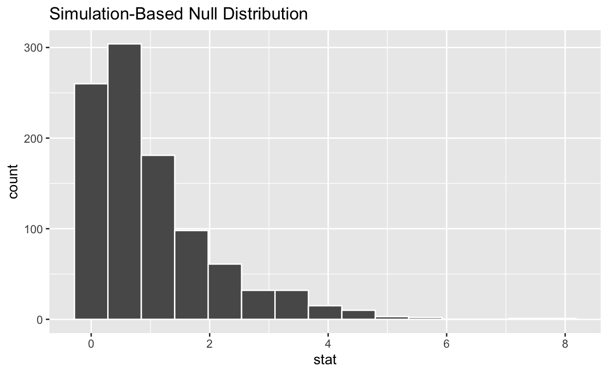
# … with 990 more rows

visualize the simulated null distribution

visualize(null_distribution_anova)

calculate the statistic from your observed data

Assign the output observed_f_sample_stat
Display observed_f_sample_stat

observed_f_sample_stat  <- hr_anova %>%
  specify(response = hours, explanatory = status)  %>% 
  calculate(stat = "F")

observed_f_sample_stat

Response: hours (numeric)
Explanatory: status (factor)
# A tibble: 1 × 1
   stat
  <dbl>
1  128.

get_p_value from the simulated null distribution and the observed statistic

null_distribution_anova  %>% 
  get_p_value(obs_stat = observed_f_sample_stat, direction = "greater")

# A tibble: 1 × 1
  p_value
    <dbl>
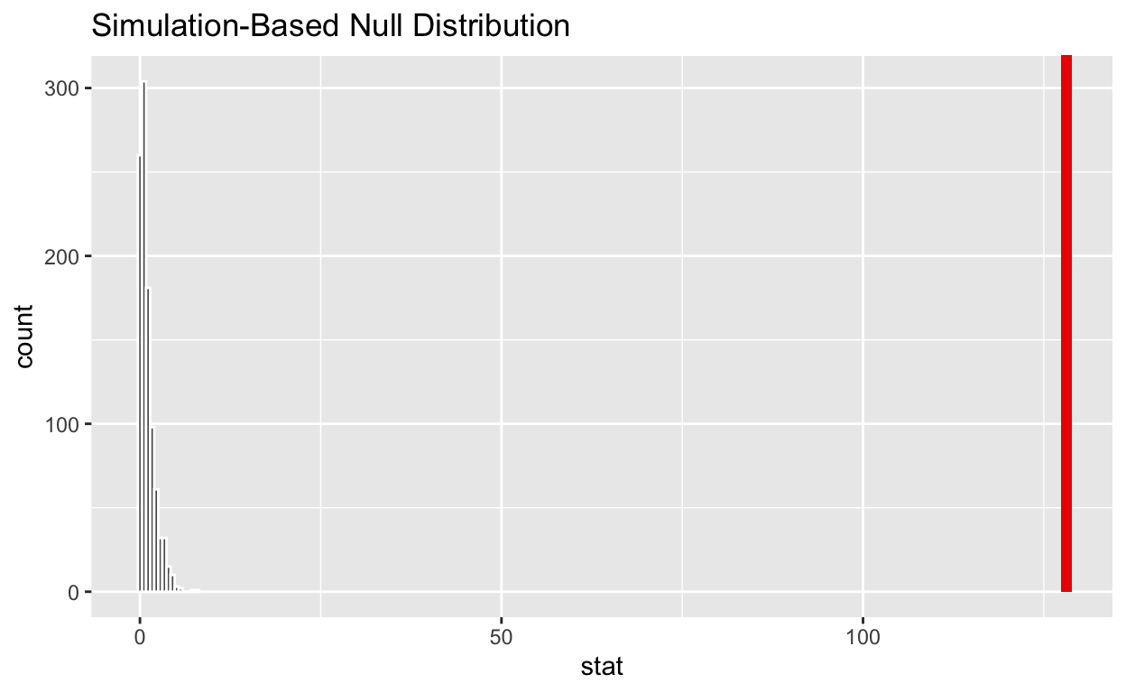
1       0

shade_p_value on the simulated null distribution

null_distribution_anova  %>% 
  visualize() +
  shade_p_value(obs_stat = observed_f_sample_stat, direction = "greater")

Hypothesis Testing

T-Test

Use skim to summarize the data in hr

specify that hours is the variable of interest

hypothesize that the average hours worked is 48

generate 1000 replicates representing the null hypothesis

calculate the distribution of statistics from the generated data

visualize the simulated null distribution

calculate the statistic from your observed data

get_p_value from the simulated null distribution and the observed statistic

shade_p_value on the simulated null distribution

Is the average number of hours worked the same for both genders in hr_2

Use geom_boxplot to plot distributions of hours worked by gender

specify the variables of interest are hours and gender

hypothesize that the number of hours worked and gender are independent

generate 1000 replicates representing the null hypothesis

visualize the simulated null distribution

get_p_value from the simulated null distribution and the observed statistic

shade_p_value on the simulated null distribution

Q: Is the average number of hours worked the same for all three status (fired, ok and promoted) ?

Use geom_boxplot to plot distributions of hours worked by status

specify the variables of interest are hours and status

hypothesize that the number of hours worked and status are independent

generate 1000 replicates representing the null hypothesis

calculate the distribution of statistics from the generated data

visualize the simulated null distribution

calculate the statistic from your observed data

get_p_value from the simulated null distribution and the observed statistic

shade_p_value on the simulated null distribution